Understanding Parabolic Mirrors for Radio Telescopes

In the realm of radio telescope construction, the principles of parabolic geometry play a crucial role. This article aims to simplify the theoretical aspects of parabola design, providing insights into how these structures function in capturing radio waves from celestial sources.

Grasping the Parabola

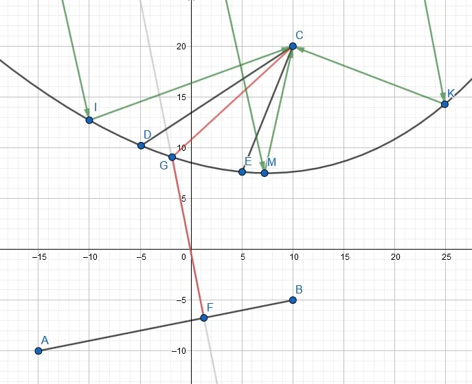
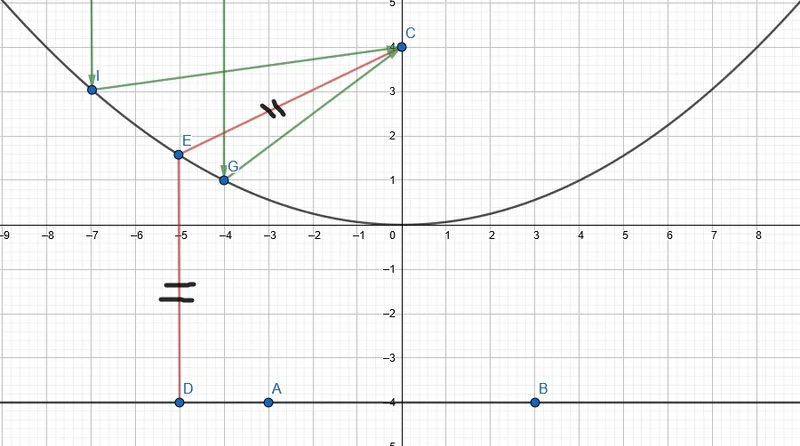
To create a parabolic mirror, one must establish a directrix line, referred to as (A, B), and a focal point denoted as C. The directrix is oriented perpendicularly to the incoming rays that the telescope aims to observe, effectively directing them towards the source.

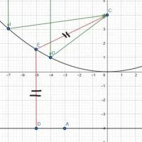
A key characteristic of a parabola is that the lengths of the segments EC and ED must be equal. This equality defines the parabolic shape, ensuring that all incoming rays (illustrated in green) are reflected towards the focal point.

Establishing the Parabola with a Central Receiver

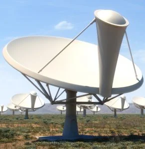
In this configuration, the antenna features a centrally located receiver, representing a prime focus setup. This arrangement simplifies the calculations involved.

Starting with 2D Calculations

For this example, let us position the focal point at (0, 4), which is 4 meters from the parabola's center. The directrix will then be located at -4 meters, functioning as a line (or a plane in 3D) perpendicular to the rays we wish to receive, referred to as d.

To maintain the condition EC = ED, we apply the distance formula derived from the Pythagorean theorem:

(x1–x2)² + (y1–y2)²

where (x1, y1) represents a point on the parabola and (x2, y2) corresponds to the focal point.

The distance for EC is calculated as:

(x – 0)² + (y – 4)²

ED remains perpendicular to the directrix as it points towards the source that the parabola is designed to capture, allowing us to eliminate x from the formula for ED.

ED = (y – (–4))²

With EC and ED established, we seek to express y in terms of x under the condition EC = ED:

(y – (–4))² = (x – 0)² + (y – 4)²

After simplification, we arrive at:

(y + 4)² = x² + (y – 4)² y² + 8y + 16 = x² + y² – 8y + 16

This leads to:

16y = x² y = x² / 16

Using this formula, one can accurately position points on the parabola for a focal point located 4 meters away.

Expanding to 3D Calculations

When considering a focal point at (0, 4, 0), the equation adapts to:

(y – (–4))² = (x – (0))² + (y – 4)² + (z – 0)² y² + 8y + 16 = x² + y² – 8y + 16 + z²

y = (z² + x²) / 16

For instance, to find the point of the parabola at (1, 1), we calculate: m = 0.125m = 12.5cm

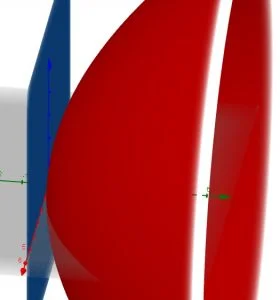
Thus, the point of the parabola located 1 meter horizontally and 1 meter vertically will be positioned 12.5 cm from the blue plane.

Establishing the Parabola with an Off-Center Receiver and Slanted Directrix

This telescope configuration features a receiver that is offset from the center, known as an offset configuration.

The calculations become slightly more complex but adhere to the same foundational principles.

2D Calculations for Offset Configuration

With a focal point at (10, 20), we begin by determining the equation for the directrix: y = ax + b where a = (y1 – y2) / (x1 – x2) and b = y2 – ax2.

Using points A(-15, -10) and B(10, -5), we find: a = (–10 – (–5)) / (–15 – 10) a = –5 / –25 a = 0.2

Substituting back, we calculate: b = –5 – (0.2 * 10) b = –7

Thus, the equation for the directrix becomes: y = 0.2x – 7

Next, we revisit the parabola's equation: (y – (0.2x – 7) + 0.2x – 75)² + (y – (0.2(y – (0.2x – 7) + 0.2x – 75) + x) – 7)² = (x – 10)² + (y – 20)²

Using computational tools like Wolfram Alpha, we isolate y: y = 512(–12x – 25x² + 2177 – 30x + 1670)

For the 3D representation: (y – (0.2x – 7) + 0.2x – 75)² + (y – (0.2(y – (0.2x – 7) + 0.2x – 75) + x) – 7)² + (y – (0.2(y – (0.2z – 7) + 0.2z – 75) + z) – 7)² = z² + (x – 10)² + (y – 20)²

Wolfram yields: –0.96x² – 0.384xy + 17.2x + 0.8832y² – 0.384yz + 66.88y – 0.96z² – 2.8z – 402 = 0

This can be further simplified to: –0.96x² + 17.2x – 0.96z² – 2.8z – 402 = y(0.96x + 0.96z + 17.2) – 0.384y²

With a simple Python script, one can derive the coordinates necessary to construct the parabolic reflector.